Amazon Reviews Sentiment Analysis Using Machine Learning Classification Algorithms

Contents

1. Dataset

2. The model

   2.1 Feature engineering with TfidfVectorizer and stop words

   2.2 Classification models: Logistic Regression and Linear Support Vector Machine

   2.3 Building the Model

   2.4 Model Evaluation

3. Summary

The aims of this analysis are to determine what keywords are most associated with positive and negative reviews and to create a model that is able to classify a review of books. By determining what aspects of the review that is important, we are able to focus on them to enhance the user experience. We are also able to live monitor social media conversation and live reviews to gauge consumer satisfaction.

The dataset used is 142.8 million reviews of 212,404 unique books from 1996-2014. Three categories will be used: History, Cooking, and Business and Economics. Overall, there are certain useful keywords that are associated with positive or negative reviews that can be used to give an idea of what customer deems important. The models are able to achieve around 85-88% average accuracy in classifying whether a review is positive or negative.

1. Dataset

Fig 1. Difference between summary and text review

The dataset has three main features of interest: review score, summary, and text review. The difference between summary and text review is shown in Fig 1. In total, there are 89,988 unique History books, 65,618 Business and Economics, and 29,985 Cooking books that will be used in the model. The reviews will be classified into positive for 4 and 5 stars, and negative for 1-3 stars. In practice it is possible to use sentiment analysis to classify into more categories, such as determining whether a consumer review is an issue with packaging, wrong order, or defects. But with our purposes, and reviews classification in general, determining whether a review is positive or negative is a good approach. From here I will only show the codes for the History category, though changing the codes will work by changing the category for the other two. We will perform the analysis on the text and summary review.

import pandas as pd

#the category is in a different file, we must merge the two
df1 = pd.read_csv('data/Books_rating.csv')
df2 = pd.read_csv('data/books_data.csv')

df_merged = pd.merge(df1, df2, how='inner',on=['Title'])
df_merged = df_merged[["review/score",'review/summary', 
                       'review/text','categories']] #selecting the necessary columns

history = df_merged.loc[df_merged['categories']=="['History']"] #filtering by the History category

import numpy as np
history['class'] = np.where(history['review/score']>3, 1, 0) #creating positive and negative class

history["review/summary"].astype(str)
history["review/text"].astype(str)

#creating the datasets for the model
X_sum = history["review/summary"]
y_sum = history["class"]

X_text= history["review/text"]
y_text = history["class"]

The reviews for the three categories are highly skewed towards five stars, as shown in in Fig 2. For Business and Economics, 5 stars make up 59.6% of the reviews, 58.4% for History, and 69% for Cooking.

import seaborn as sns
sns.histplot(history['review/score'],stat="probability",discrete=True).set_title('History book reviews distribution')

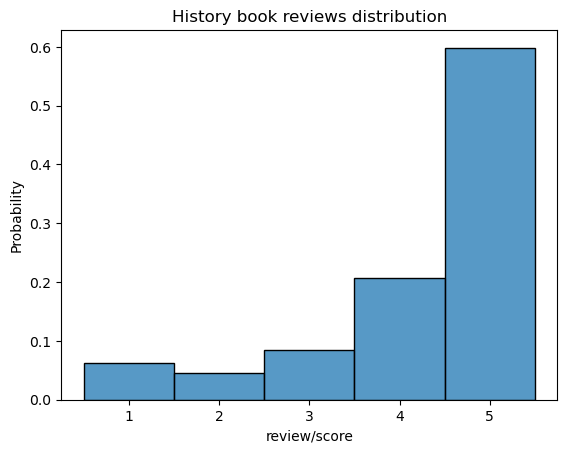
Fig 2. Reviews distribution

This skewness has an interesting impact towards the result. The keywords associated with positive reviews are more generic and less informative compared to the negative reviews. A reason for this is because simply there are more variation of different words for positive reviews, which makes the model harder to pinpoint on some specific keywords, while its less for negative reviews and thus they are more clustered and focused on certain keywords. It is also possible that people that left negative reviews have a specific reason for their displeasure and thus certain keywords will appear more frequently.

2. The model

We will use scikit-learn to analyse the dataset. First, I will explain the tools that will be used, TfidfVectorizer for feature engineering, and Logistic Regression as the classifiers. Overall the model has reasonable accuracy at around 85-88%, while we are able to extract certain keywords that are associated with whether the review is a positive or negative.

2.1 Feature engineering with TfidfVectorizer and stop words

Transforming the data is necessary into a form that the ML algorithms understand. For natural language processing, an algorithm to do this is the TfidfVectorizer. A basic approach to transforming text data is to count how many word appears. However, this runs into the issue of some common words appear more often that do not give any meaningful sentimental context but are considered important just because they appear often. There are two ways to handle this problem: with Tfidfvectorizer and stop words.

What TfidfVectorizer does is to normalise the frequency of words by putting more weight to words that appear less in different instances. In the context of reviews, words that often appear in different reviews are considered to be less important, while words that appear less is considered more important. This is useful because TfidfVectorizer is able to eliminate some unimportant words by putting more weights to unique words. Another way to eliminate words is to pass stop words, which tells the model to ignore some words entirely. scikit-learn has a built-in stopwords list called english, which consists of common uninformative words, such as the, and, if, etc. We will see both of these methods in action later.

2.2 Classification models: Logistic Regression

A logistic regression model is a tool that can be used as a classification algorithm, in this case whether a review is positive or negative. It is a relatively simple model compared to more complicated ensemble classifiers, such as Random Decision Trees Classifier or Gradient Boosting Classifier. Nontheless its still a good place to start and the models we will develop have reasonable accuracy at around 85-88%.

An important adjustable hyperparameter for logistic regression is C. Essentially this adjusts the decision boundary so that it either prioritise the majority of the data points or that individual data point is classified correctly. For higher C value we would force the model to classify the individual data points as correctly as possible, while we would expect a smaller value to be less sensitive towards outliers. We will see that this hyperparameter is adjustable and scikit-learn can iterate values that give the best accuracy of the model.

2.3 Building the Model

The main backbone of the model is pipe , which allows us to first transform the data using TfidfVectorizer and feed them into the Logistic Regression model in a single go, thus streamlining the process, reduce the likelihood of error, and improve readability.

from sklearn.feature_extraction.text import TfidfVectorizer
from sklearn.pipeline import make_pipeline
from sklearn.linear_model import LogisticRegression
from sklearn.model_selection import GridSearchCV
from sklearn.feature_extraction.text import ENGLISH_STOP_WORDS

pipe = make_pipeline(TfidfVectorizer(min_df=10, stop_words=('english','disappointment','disappointed','disappointing')),
                     LogisticRegression())
param_grid = {'logisticregression__C': [0.001, 0.01, 0.1, 1, 10]}
grid = GridSearchCV(pipe, param_grid, cv=5, n_jobs=-1)

makepipeline first transform the data using TfidfVectorizer. The min_df parameter sets the minimum amount of a word that must occur to be incorporated into the model. We use the scikit-learn built in stop words function, and added 4 more words. Without these 4 words the model put too much strength on those words but they do not really mean anything if we want to extract certain attributes that are deemed important. The results without these 4 stop words will be shown later when we discuss the results.

By passing these stopwords, we are able to reduce the number of features from 3722 to 3482 by

print(repr(X_sum_result))
<89988x3722 sparse matrix of type '<class 'numpy.float64'>'
    with 389562 stored elements in Compressed Sparse Row format>

Adding the 4 variations of disappoint will reduce the features from 3722 to 3718, as expected. X_sum_result will be discussed later when we extract the coefficients.

paramgrid lists all the discussed C hyperparameters for the logistic regression. The GridSearchCV then runs the model with all these different hyperparameters, after which we can extract which one has the highest accuracy using .best_score_. The parameter cv sets the cross-validation iteration number, while n_jobs sets the amount of cores the CPU uses to run the model, setting it to -1 uses all the available cores, which is able to exponentially speed up the process.

Running this model by

sum_model = grid.fit(X_sum, y_sum) 
sum_model = grid.fit(X_text, y_text)

and showing the results

print(sum_model.best_score_)
0.8474

Summarising the results for all of the categories:

• Summary History: 0.8474

• Text History: 0.8731

• Summary Business and Economics: 0.8319

• Text Business and Economics: 0.8641

• Summary Cooking: 0.8774

• Text Cooking: 0.90255

In general the text model outperform its summary model counterpart, which is to be expected as there are more features for the text model, thus the text model have more data to be trained with.

Extracting the coefficients into a pandas dataframe is a bit tricky. The numerical values can be easily extracted by using .best_estimator, but to get the coefficient names, we need first transform the original X_sum using the TfidfVectorizer from our model. This would then get sorted in a descending order, and the combined using pd.concat with .best_estimator of the logistic regression model. Because the .best_estimator sort the coefficient values in a descending order, this new dataframe will exactly match the coefficient names and their value.

text_vectorizer = text_model.best_estimator_.named_steps['tfidfvectorizer']

X_text_result = text_vectorizer.transform(X_text)

text_max_value = X_text_result.max(axis=0).toarray().ravel()
text_sorted_by_tfidf= text_max_value.argsort()
text_feature_names = np.array(text_vectorizer.get_feature_names_out())

text_coefficients = pd.concat([pd.DataFrame(text_feature_names),
                          pd.DataFrame
                          (np.transpose(text_model.best_estimator_.named_steps
                                        ['logisticregression'].coef_))], 
                         axis = 1, )
text_coefficients.columns=['feature','coef']

Finally, the top and lowest 20 coefficients for all the categories are

Summary Business and Economics Top 20

Summary History Top 20

Text Cooking Top 20

Summary Business and Economics Lowest 20

Summary History Lowest 20

Text Cooking Lowest 20

Summary Cooking Top 20

Text Business and Economics Top 20

Text History Top 20

Summary Cooking Lowest 20

Text Business and Economics Lowest 20

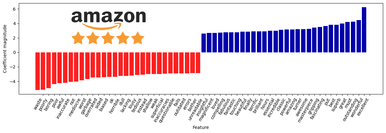
Text History Lowest 20

These can also be visualised as so

Summary Business and Economics

Text Business and Economics

Summary History

Text History

Summary Cooking

Text Cooking

2.4 Model Evaluation

As suggested earlier, specific keywords that are crucial in understanding certain reviews appear more frequently in the negative reviews. A main reason for this is that there are more positive reviews, different words appear more frequently, and thus the model picks up more, generic, positive terms. This is fine if the aim for the model is to classify whether a review is positive or negative. In fact, by picking up a more varied vocabulary the model can better classify whether the review is negative or positive. 

Fig 3. Variations of disappoint are now in the top 5 in summary Cooking reviews

If, on the other hand, that only a smaller vocabularies are used, there is less scope for the model to pick up certain keywords. This is a main reason why we dropped the words “disappoint”, “disappointed”, and “disappointment” because they are considered to be really strong by the model, as seen in Fig 3.

But if the main purpose is to assess important keywords, adding words that are really uninformative will distort the analysis. For example the terms ‘errors’ and ‘lacking’ are not found in Fig 3, but are found in ‘Summary Cooking Lowest 20’.

The purpose of the model is more crucial as we can put even more stopwords of generic uninformative keywords, which would mean that the model would pick up even more informative keywords. The tradeoff though is that the model accuracy would drop further. Adding the 4 variations of ‘disappoint’ reduced the accuracy by 1-1.5%.

A middle ground approach is to adjust the stopwords such that it provides the best accuracy as possible, and then to filter out the generic terms so that we are able to extract the most informative ones. This would put more importance to more uninformative words, but is necessary if we do not have labelled data, such as monitoring social media chatters.

Nonetheless, the model is able to pick up certain useful keywords that are indicative of whether a review is positive/negative. For example, looking at both the negative summary and text history reviews, we are able to see that accuracy and bias are important in understanding why readers left negative reviews. In summary and text cooking reviews, meanwhile, we can see that simplicity and deliciousness of food are important in positive reviews.

These results can be used as indicators of what features should be focused on. Ensuring that writing a cook book that is simple and that produce delicious food mean that the customer is more likely to leave a positive review. We can extent this model easily to any data that involve text processing. The more niche the data that we process, the more likely that certain keywords will appear more that are relevant.

We can also use the model as a live tracker of reviews to track whether the product is received well or not, and whether the strategy of focusing on certain aspects works or not.

3. Summary

We have developed a sentiment analysis model using TfidfVectorizer and Logistic Regression on Amazon book text and summary reviews of 3 categories. The model achieved a reasonable accuracy, about 85-88% in average, meaning that it can perform well in classifying whether a review is negative or positive. We also discovered that there are certain keywords that influence whether a review is negative or positive, meaning that we can gain an insight of what aspect of a product should be focused on.

A further iteration of this project may be to try different algorithms, especially with ensemble methods to assess whether there is a boost in accuracy, although this may only be a few percents without further feature engineering, and whether other keywords may appear that are more indicative of whether a review is positive or negative.